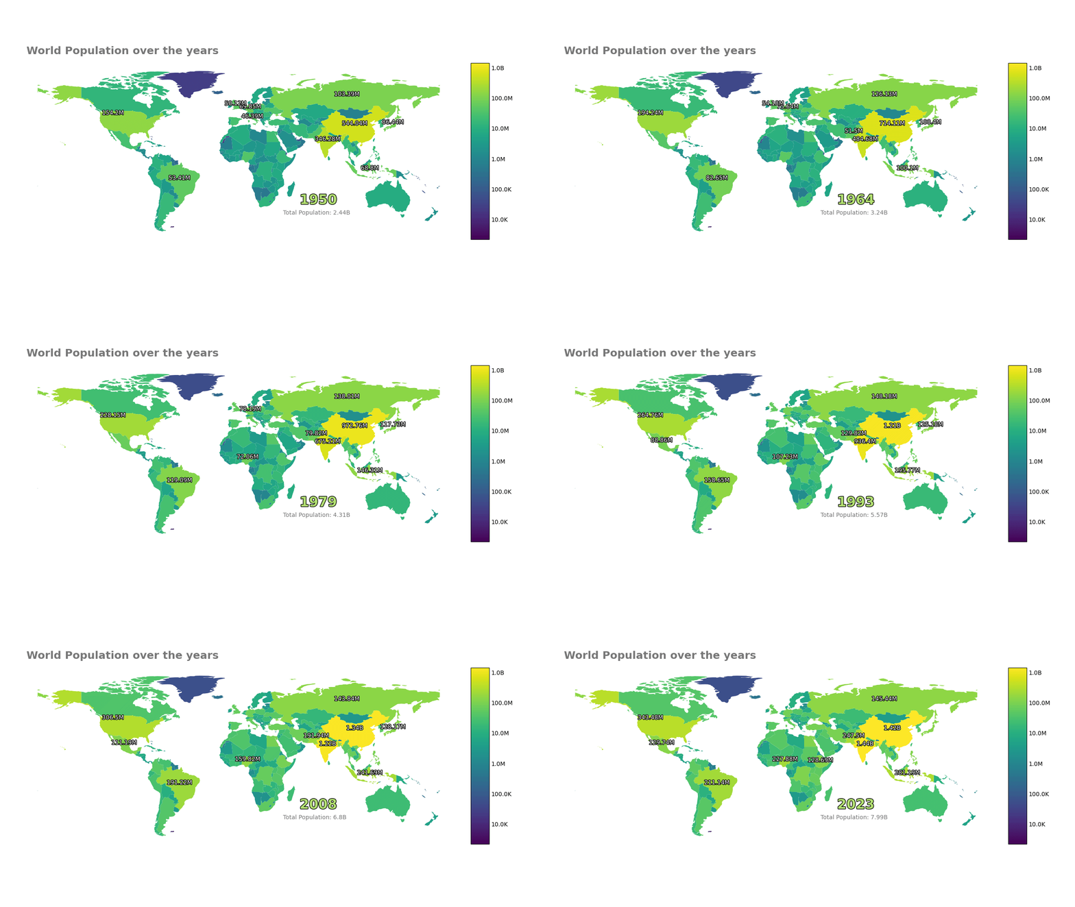
Creating an Animated Choropleth

The data

For the map data we will be using Natural Earth — Admin 0 – Countries. Click the download countries and grab the ne_110m_admin_0_countries. For the population data we will be using ourworldindata population data, grab the full data with around 19k rows.

Some of the displayed tables are shortened for easier understanding, you will get a larger table trying to replicate this.

Converting long data to wide data

df = pd.read_csv('data/population.csv')
df.head()

#	Entity	Code	Year	Population
0	Afghanistan	AFG	1950	7,776,180
1	Afghanistan	AFG	1951	7,879,343
2	Afghanistan	AFG	1952	7,987,784
3	Afghanistan	AFG	1953	8,096,703
4	Afghanistan	AFG	1954	8,207,954

We will be joining both the population and map data on the Country ISO_A3 code column, so better to remove any nan code(ISO_A3) before hand.

df.isna().sum()

>>>
Entity         0
Code         592
Year           0
all years      0
dtype: int64

df = df.dropna()

Now for the important part, unlike the rest of the library, time variable here is kept as individual columns and not as a single column/index. This design choice was chosen so it is easier to work with geopandas as geopandas requires all geometries in a column to work.
In a nutshell previously we had.

        [other var]
           |
           |
[Time]--- [value]

For choropleth we have the following wide-data format.

              [Time]
                |
                |
[Geometry]--- [value]

So we will pivot it like this:

df = df.pivot(index=['Entity','Code'], columns='Year', values='all years').reset_index()
df.head()
df.to_csv("pivot_population.csv",index=False)

#	Entity	Code	1950	1951	1952	1953	1954	1955	1956	1957
0	Afghanistan	AFG	7,776,180	7,879,343	7,987,784	8,096,703	8,207,954	8,326,981	8,454,303	8,588,340
1	Africa	OWID_AFR	227,776,838	232,557,370	237,539,910	242,685,417	248,006,203	253,538,234	259,271,764	265,129,059
2	Africa (UN)	UN_AFR	227,776,420	232,556,973	237,539,543	242,685,066	248,005,819	253,537,849	259,271,438	265,128,663
3	Albania	ALB	1,247,854	1,276,365	1,308,368	1,343,581	1,381,088	1,418,855	1,456,823	1,497,954
4	Algeria	DZA	9,018,423	9,269,870	9,521,212	9,772,644	10,014,393	10,247,429	10,482,183	10,717,503

Which gives us 254 regions over 74 years, as you can see not all regions here are countries.

df.shape
(254, 76)

Reading the shp file

We will be using geopandas for all the 'maplysis' stuff.

mapdf = geo.read_file('ne_110m_admin_0_countries.shp')
mapdf.head()

#	featurecla	scalerank	LABELRANK	SOVEREIGNT	SOV_A3	ADM0_DIF	LEVEL	TYPE	TLC	ADMIN	geometry
0	Admin-0 country	1	6	Fiji	FJI	0	2	Sovereign country	1	Fiji	MULTIPOLYGON (((180 -16.067, 180 -16.555, 179....
1	Admin-0 country	1	3	United Republic of Tanzania	TZA	0	2	Sovereign country	1	United Republic of Tanzania	POLYGON ((33.904 -0.95, 34.073 -1.0598, 37.699...

We only care about the Geometry for plotting and ISO_A3 for joining.

mapdf = mapdf[["ISO_A3","geometry"]]
mapdf.head()

#	ISO_A3	geometry
0	FJI	MULTIPOLYGON (((180 -16.067, 180 -16.555, 179....
1	TZA	POLYGON ((33.904 -0.95, 34.073 -1.0598, 37.699...
2	ESH	POLYGON ((-8.6656 27.656, -8.6651 27.589, -8.6...
3	CAN	MULTIPOLYGON (((-122.84 49, -122.97 49.003, -1...
4	USA	MULTIPOLYGON (((-122.84 49, -120 49, -117.03 4...

There are additional region / country in both data, I will leave exploring that as an assignment.

df.shape, mapdf.shape
>>>((254, 76), (177, 2))
len(set(mapdf.ISO_A3).intersection(set(df.Code)))
>>170

Merging both data to get our desired wide-data format. We are doing an Inner join to get the common countries in both data.
note - unlike population data, mapdata here only contain countries.

mapdf.columns = ["Code", "geometry"]
mapdf = pd.merge(mapdf, df, how='inner', on=['Code'])
mapdf.to_csv("pop.csv",index=False)
mapdf.shape

(170, 77)

Our expected wide-data format: We have got our geometry column, time unit as columns and additional information variables like entity. Now onto the animation plotting.

#	Code	geometry	Entity	1950	1951	1952	1953	1954	1955	1956
0	FJI	MULTIPOLYGON (((180 -16.067, 180 -16.555, 179....	Fiji	309,525	316,137	323,374	331,225	339,754	349,084	359,218
1	TZA	POLYGON ((33.904 -0.95, 34.073 -1.0598, 37.699...	Tanzania	7,625,152	7,812,973	8,009,083	8,213,117	8,424,792	8,644,856	8,874,780

Using Pynimate Choropleth

First convert the geometry strings (we are reading them as strings initially) into objects.

mapdf["geometry"] = mapdf["geometry"].apply(wkt.loads)
mapdf = geo.GeoDataFrame(mapdf, geometry=mapdf.geometry)

We will be using pynimate.Choropleth for setting up our Choropleth plot.

The from_widedf() constructor is handy here for easily passing the wide-data without creating a GeoDatafier.

Argument	Value	Description
`data`	`data`	Our created wide-format data
`time_format`	`"%Y"`	The data contains year-only time values, like '1991', '1992' etc
`ip_freq`	`"6MS"`	We interpolate every 6 months for a smoother animation
`log_norm`	`True`	The country-wise population data is highly skewed, so we use a logarithmic scale for better visualization

The annot_geo parameters are interesting.
annot_geo_masks parameter is used to specifically include or exclude (prefix column name with ~) rows. Here we are excluding population of geometry 'BGD' (Bangladesh) from being annotated throughout the animation, as it is overlapping with India.

Parameter annot_geo_filter on the other hand is used to filter 'n' values of each time column, in this case we are keeping only top 10 most populous country for any time frame.

canvas = nim.Canvas()
plot = nim.Choropleth.from_widedf(
    data,
    "%Y",
    "6MS",
    log_norm=True,
    annot_geo_masks={"~Code": ["BGD"]},
    annot_geo_filter=top_n(10),
)

Some more theming and customizations.

plot.set_title(
    "World Population over the years",
    0.02,
    1.05,
    size=18,
    color="#777777",
    weight=600,
)

The code snippets below are good examples on how to utilize the callback features.
For instance, here the api exposes time frame i and datafier dfr.

The below snippet utilizes this to show the world population of a time frame (6 months for our case)
First we take the sum of a column / time frame, get the human_readable string of it, like 2.5m,etc and add some an string literal like 'Monthly Total: 2.5K'

"".join(("Monthly Total: ", human_readable(dfr.data[dfr.time_cols[i]].sum()))

plot.set_text(
    "time",
    callback=lambda i, dfr: dfr.time_cols[i].strftime("%Y"),
    x=0.8,
    y=0.3,
    size=23,
    color="#b3df72",
    weight=800,
    ha="center",
    path_effects=[pe.withStroke(linewidth=2, foreground="black")],
)

plot.set_text(
    "sum",
    callback=lambda i, dfr: "".join(
        ("Monthly Total: ", human_readable(dfr.data[dfr.time_cols[i]].sum()))
    ),
    x=0.68,
    y=0.24,
    size=10,
    color="#777777",
    weight=200,
)

Finally we save the animation.

canvas.add_plot(plot)
ani = canvas.animate(interval=200)
canvas.save("ma2", fps=24, extension="mp4")
plt.show()

As you can see, majority of the work is performing the data transformation.
Pynimate makes rest of the animation process very simple.

Creating an Animated Choropleth

The data

Converting long data to wide data

Reading the shp file

Using Pynimate Choropleth

Result!